💻 XAIoWeb
XAIoWeb is a web interface executed in local mode (127.0.0.1:8080) that allows to visualize the results of the
explainability and fairness methods after executing the fit() methods of the Explainer,
Why or Fairness classes of XAIoGraph.
A sequence of JSON files are generated in the xaioweb_files folder after executing the fit() method of the
Explainer, Why or
Fairness classes (folder name is specified in the class constructor’s
destination_path parameter). Web interface displays the outcomes using the following JSON files:
JSON FILE NAME |
|---|
global_explainability.json |
global_target_distribution.json |
global_graph_description.json |
global_graph_nodes.json |
global_graph_edges.json |
global_heatmap_feat_val.json |
global_target_explainability.json |
local_dataset_reliability.json |
local_reason_why.json |
local_graph_nodes.json |
local_graph_edges.json |
fairness_confusion_matrix.json |
fairness_highest_correlation.json |
fairness_independence.json |
fairness_separation.json |
fairness_sufficiency.json |
fairness_sumarize_criterias.json |
Warning
If any of these files are not generated, the website will not display the results.
To launch the web (with the virtual environment enabled), run the following command:
>> xaioweb -d xaioweb_files -o
This command takes the following parameters:
-do--data[REQUIRED]: JSON files path-po--port[OPTIONAL]: Web server port. 8080 by default-oo--open[OPTIONAL]: Open web in browser-fo--force[OPTIONAL]: Force building the web from scratch, overwriting the existing one
If executed with the -o option, the web browser (127.0.0.1:8080) will be opened with XAIoWeb:
Warning
After launching the web, a hidden folder (.xaioweb) containing the web files will be generated.
Each of the XAIoWeb sections is shown below, along with an explanation of each of its graphics:
Note
All images shown in the documentation in this section are from the titanic example.
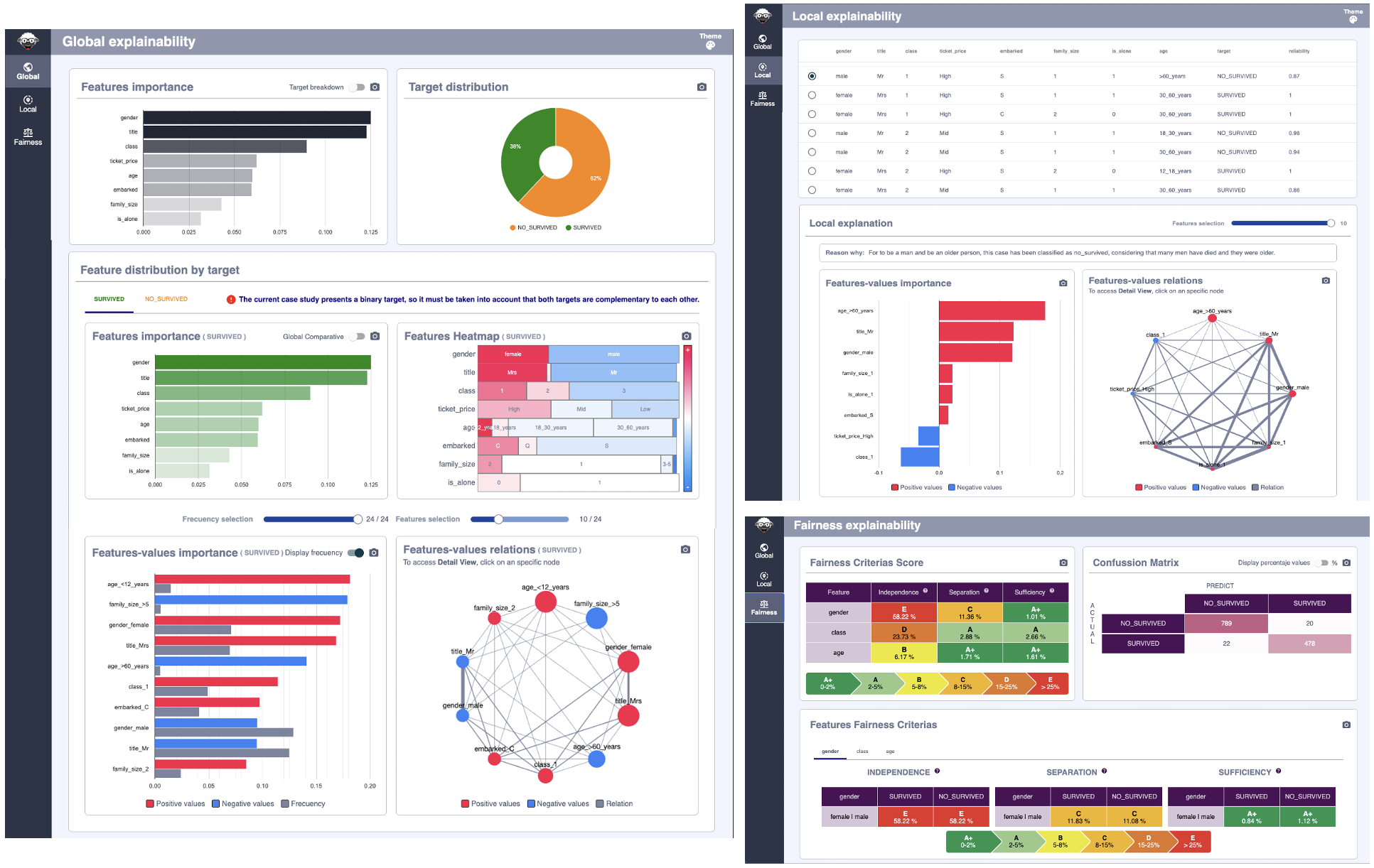
Global Explainability
The Global module presents a statistical calculation on the main characteristics of the dataset.
It must be understood that all entries in the dataset are analyzed individually and their statistics are subsequently aggregated in this module.
It is important to understand that the results are presented at the level of the entire dataset and according to the different targets that make it up.
The page is divided into two major sections, the top (formed by the Features Importance and Target distribution graphs) displays the information of the entire dataset. The bottom, under the title “Feature distribution by target”, shows the features information for a specific target, displaing consolidated calculations grouped by the target value.
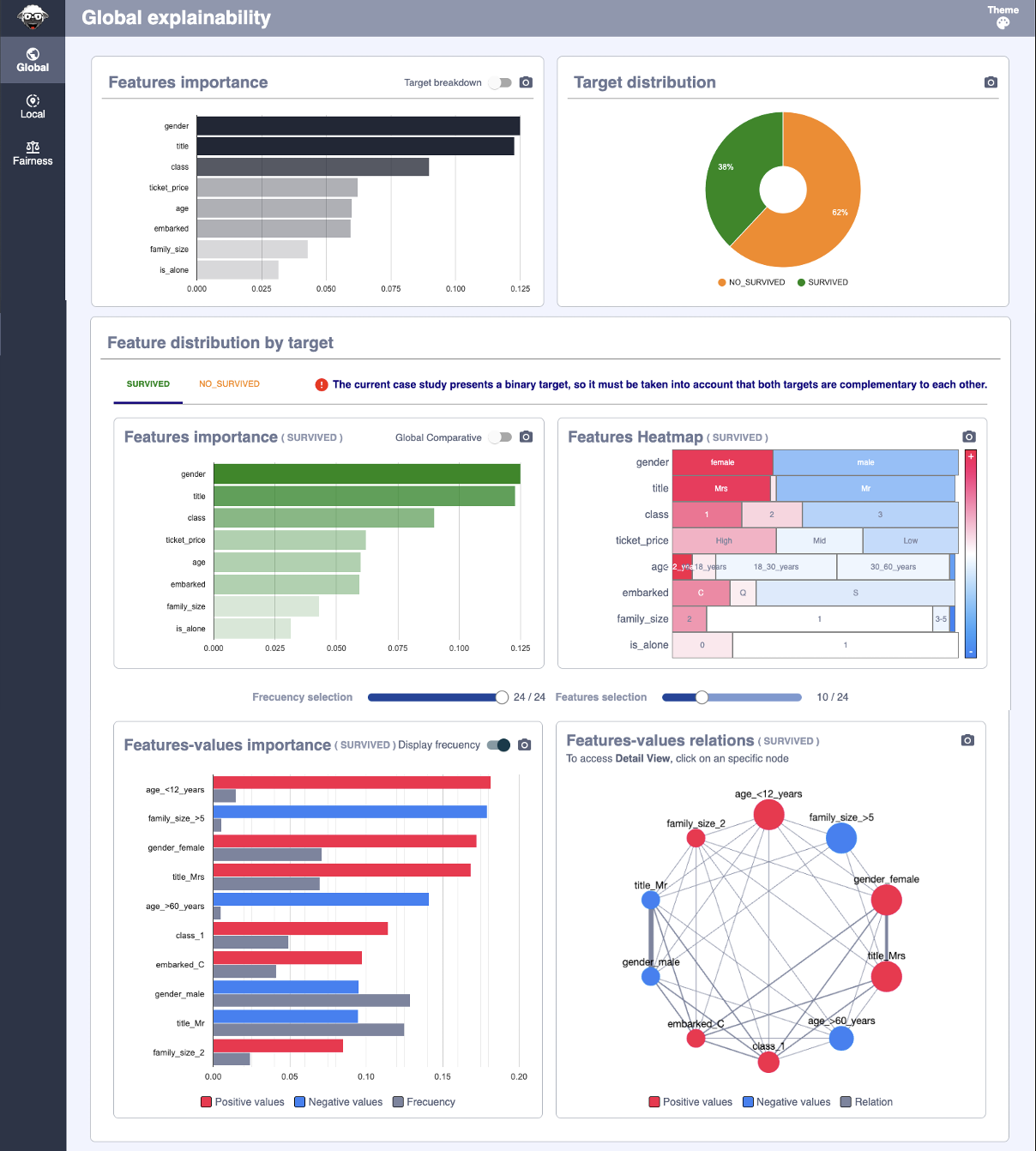
Next, we will look at each of the graphs that make it up and its meaning.
Features importance
This graph displays at a general level (regardless of the target) the importance ordered downward of each of the features of the dataset. The importance of these is represented, not only by the length of the horizontal segment but also by its opacity level.
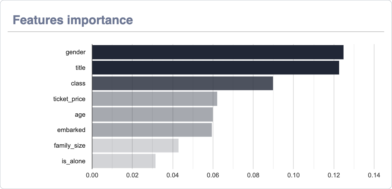
Notice that in the upper right corner of the chart, next to the export function, we have a switch that allows you to show the breakdown of values according to the target.

As an important note, the colors of the targets that the graph located to the right (Target distribution) have beenined to facilitate their reading. The X-axis has also been removed as the numerical values are different from the aggregate view (as the representative is the size of the horizontal sections) to avoid errors in the interpretation of the data.
Target distribution
This graph displays the distribution of targets across the dataset.
It is a simple statistical tool to contextualize the information contained in the dataset and visually see the importance of each of the targets.

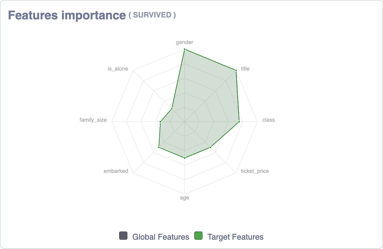
Feature importante (by target)
In this case, the graph is similar to the one located right above, but only those records have been taken into account for the selected target.
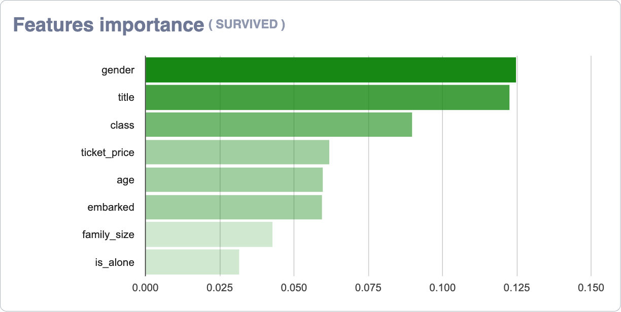
Notice that in the upper right corner of the chart, next to the export function, we have a switch that allows you to compare the values of the selected target with the general data shown in the top chart. In the specific case of datasets with binary target (there are only 2 possible values for the target) this graph will show overlapping graphs, as the average values of a target are annulled with those of the opposite.
Feature Heatmap (by target)
This graph displays a heat map with the different values that the features of the dataset can take. Those values that are most on the left will be those that contribute most positively to the target (represented by the redest color) and those located more on the right will contribute more negatively.

The different numerical values are represented depending on the opacity of the color, so that those more relevant (both positively and negatively) will have a more solid color, while those closer to the value 0 will be a more white color. The length of each of the possible values of a feature represents the number of occurrences of that value within the dataset, so that the longest values have more presence while the smallest ones have little occurrence in the data.
Features-values importance (by target)
This graph displays the specific contribution values for the feature/value pairs. This can be positive (red) or negative (blue).
It is important to note that the values shown are the same as those shown on the HeatMap.
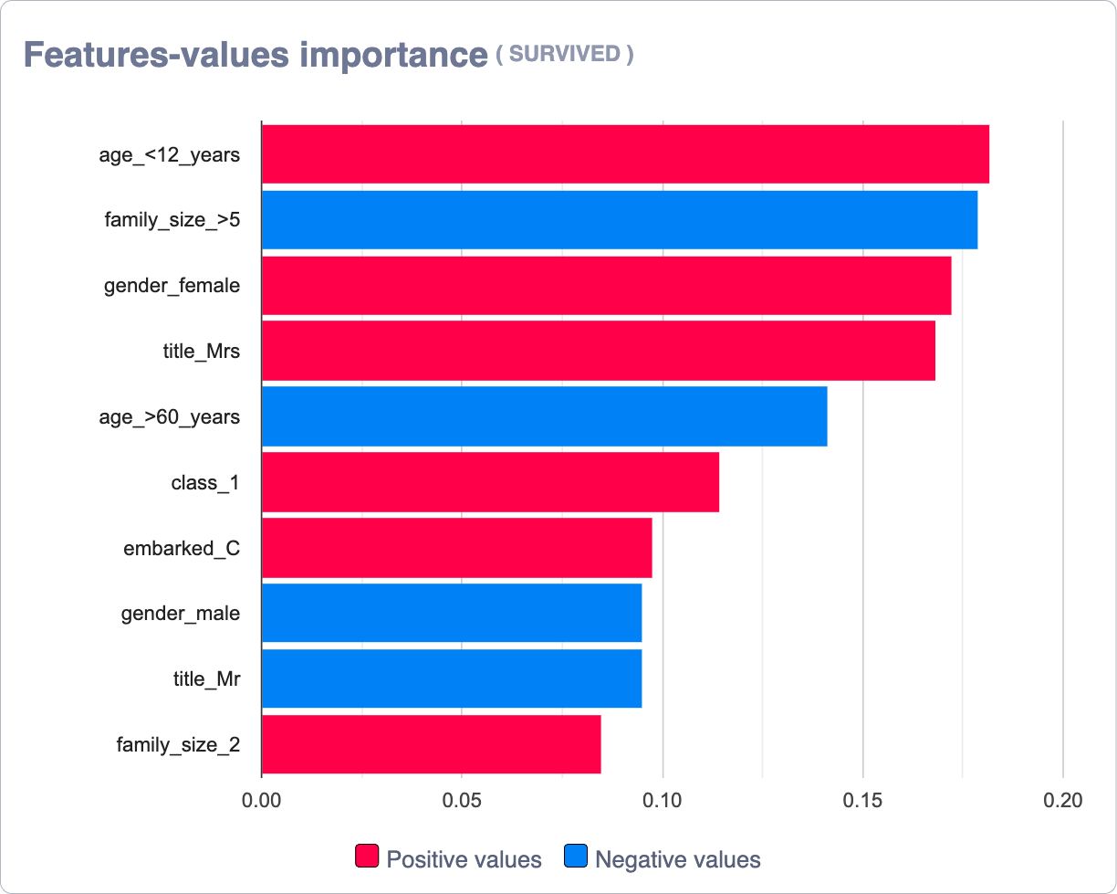
Notice that in the upper right corner of the chart, next to the export function, we have a switch that allows you to visualize the frequency of the feature-value (represented in the HeatMap by its length)

Features-values relations (by target)
This graph displays the relationships between the different features/values.

It is important to emphasize that these two last graphs are filtered thanks to sliders located just above them.

By shifting each of the bars, viewing criteria can be modified to analyze different data behaviors.
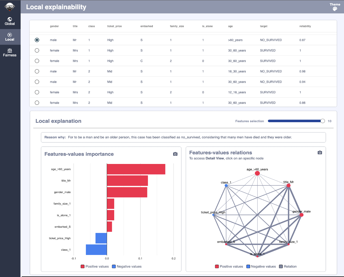
Local Explainability
The Local module presents the individual results, showing and explaining the results for a given dataset record.
Like the case of the previous module, the page is distributed into two important sections, the top presents a table with the dataset records, having by columns the different features. And the bottom that shows the calculations made for the selected record of the dataset.
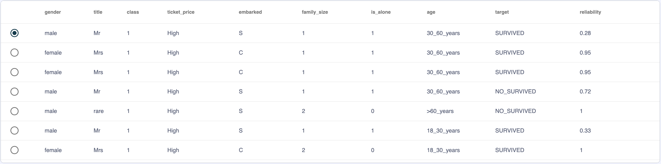
Dataset
This section displays the dataset records on which the calculations have been made, each of the features is presented in columns with the specific values taken.
It is important to note two very representative columns, the first is a checkbox that allows you to select the record on which the data is analyzed and which will be taken as a reference for the graphics located at the bottom of the screen.
And the last column called ‘reliability’, this represents a measure of the quality of the data. Since the XaioGraph does not have access to the model, it must predict the target of each record based on the analysis of the dataset, that is why there may be discrepancies between reality and prediction, and this column is what it represents, the degree of equality between the real target and the predict, which is why the records with values close to one are those in which both coincide and therefore the error dragged when generating individual calculations is much smaller.
Local Explantion (Reason Why)
This section shows a brief verbal explanation of the data that make up the record of the selected dataset. Underlining the reasons why this case has the target it has.

Features-values importance
This graph displays the specific contribution values for the feature/value pairs. This can be positive (red) or negative (blue).

Features-values relations (by target)
This graph displays the relationships between the different features/values.

It is important to emphasize that these two last graphs are filtered thanks to the slider located just above them.

By shifting the bar, the most relevant features can be displayed, so as to facilitate their reading and understanding.
Fairness
The fairness module shows the results from an ethical point of view, trying to detect possible misconduct or conditioners that can generate sensitive variables such as gender, age, etc. that can give the case of discrimination or harm.
Following the same structure as the previous modules, the page is divided into two. In the upper part we can see an analysis of all those variables detected that can constitute a case of bias and that its analysis is recommended in detail. While at the bottom, we enter the specific details of each of these variables mentioned in the top section.
To facilitate the understanding and reading of the data, a similar color scheme has been chosen to categorize the results (Fairness Category) for employees in other fields such as the Nutriscore Index in food or energy efficiency in household appliances or construction. It is a color scale from green to red. The green colors are those with values closer to 0, so they do not present relevant anomalies. While the reds are those that have exceeded a tolerance threshold and it is important to analyze them in detail.

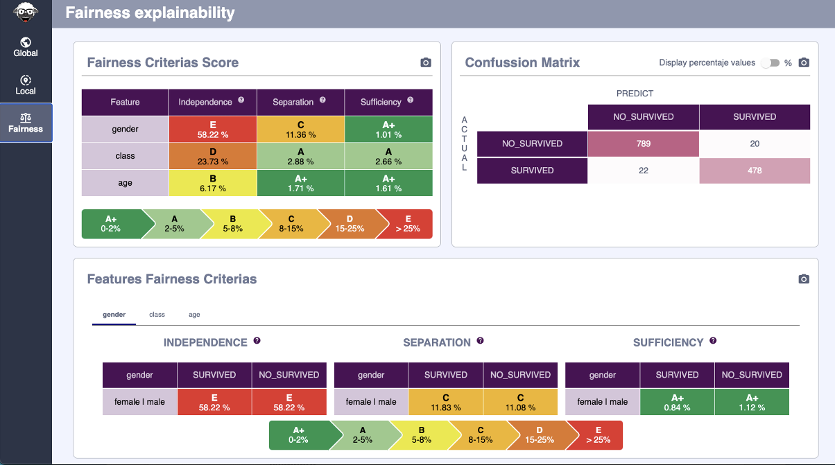
Fairness Criterias Score
This graph shows the analysis performed for each of the sensitive features based on the criteria of Independence, Separation and Sufficiency.

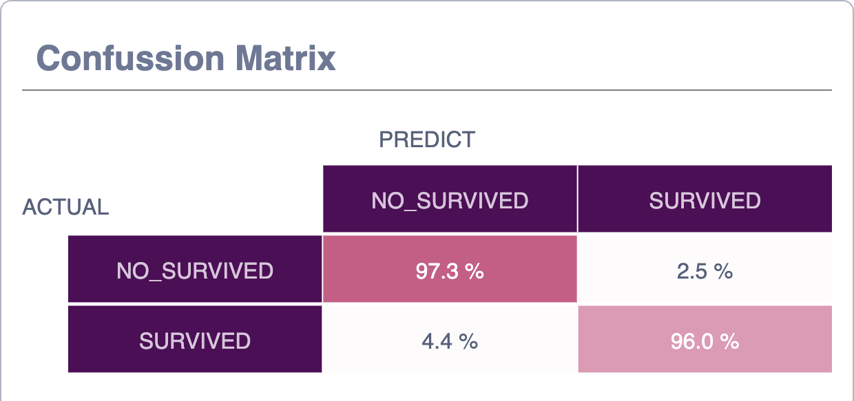
Confusion Matrix
This graph is a confusion matrix to represent the performance of the prediction algorithm.
As in any confusion matrix, columns represent the number of predictions for each target while rows represent the real class instances.
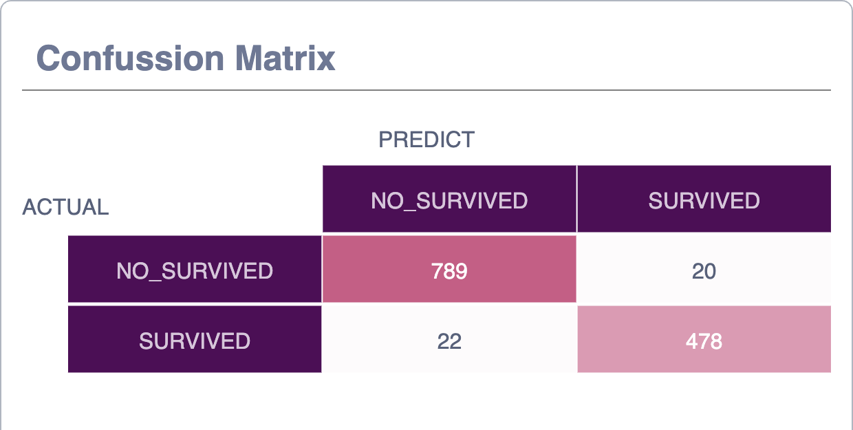
Notice that in the upper right corner of the chart, next to the export function, we have a switch that allows you to analize the numeric values or percentage values.
Features correlation (by feature)
This section displays the different degrees of correlation of the selected feature with the remaining features of the dataset, showing the Pearson correlation value

Independence, Separation & Sufficiency values (by feature)
These three graphs show the values of Independence, Separation and Sufficiency of the selected feature, making a breakdown and analysis of each of the possible values it has
