COMPAS Example#
This example highlights the most important features that the AI model considered while predicting the likelihood of
criminal recidivism. The COMPAS Dataset is used to capture the characteristics
of criminals in Broward (Florida) between years 2013 and 2014.
This dataset can be obtained using the load_compas()
function:
>>> from xaiographs.datasets import load_compas
>>> df_dataset = load_compas()
>>> df_dataset.head(3)
   id FirstName   LastName Gender        Age_range         Ethnicity  days_b_screening_arrest     c_jail_in    c_jail_out  Days_in_jail c_charge_degree                   c_charge_desc  is_recid  is_violent_recid score_risk_recidivism score_text_risk_recidivism  score_risk_violence score_text_risk_violence  Low_Recid  Medium_Recid  High_Recid  No_Recid  score_text_risk_violence  Low_Recid  Medium_Recid  High_Recid  No_Recid  Recid  predict_two_year_recid  real_two_year_recid
0   1    miguel  hernandez   Male  Greater than 45             Other                     -1.0  13/8/13 6:03  14/8/13 5:41             1               F    Aggravated Assault w/Firearm         0                 0                     1                        Low                    1                      Low          1             0           0         1                       Low          1             0           0         1      0                       0                    0
1   3     kevon      dixon   Male          25 - 45  African-American                     -1.0  26/1/13 3:45   5/2/13 5:36            10               F  Felony Battery w/Prior Convict         1                 1                     3                        Low                    1                      Low          1             0           0         0                       Low          1             0           0         0      1                       0                    1
2   5     marcu      brown   Male     Less than 25  African-American                      NaN           NaN           NaN             0               F          Possession of Cannabis         0                 0                     8                       High                    6                   Medium          0             0           1         1                    Medium          0             0           1         1      0                       1                    0
To determine the explainability of this dataset, XAIoGraphs provides a dataset that has already been discretized and
columns with targets probabilities using
load_compas_discretized() function:
>>> from xaiographs.datasets import load_compas_discretized
>>> df_dataset, features_cols, target_cols, y_true, y_predict = load_compas_discretized()
>>> df_dataset.head(3)
  id Gender        Age_range         Ethnicity MaritalStatus c_charge_degree is_recid is_violent_recid  High_Recid  Medium_Recid  Low_Recid    y_true y_predict
0  1   Male  Greater than 45             Other        Single               F       NO               NO           0             0          1  No_Recid  No_Recid
1  3   Male          25 - 45  African-American        Single               F      YES              YES           0             0          1     Recid  No_Recid
2  5   Male          25 - 45             Other     Separated               M       NO               NO           0             0          1  No_Recid  No_Recid
Code Example#
The following entry point (with Python virtual environment enabled) is used to demonstrate this example.
>> compas_example
Alternatively, you may run the code below to view a full implementation of all XAIoGraphs functionalities with this Dataset:
from xaiographs import Explainer
from xaiographs import Why
from xaiographs import Fairness
from xaiographs.datasets import load_compas_discretized, load_compas_why

LANG = 'en'

# LOAD DATASETS & SEMANTICS
df_compas, feature_cols, target_cols, y_true, y_predict = load_compas_discretized()
df_values_semantics, df_target_values_semantics = load_compas_why(language=LANG)

# EXPLAINER
explainer = Explainer(importance_engine='LIDE', verbose=1)
explainer.fit(df=df_compas, feature_cols=feature_cols, target_cols=target_cols)

# WHY
why = Why(language=LANG,
          explainer=explainer,
          why_values_semantics=df_values_semantics,
          why_target_values_semantics=df_target_values_semantics,
          verbose=1)
why.fit()

# FAIRNESS
f = Fairness(verbose=1)
f.fit(df=df_compas[feature_cols + [y_true] + [y_predict]],
      sensitive_cols=['Ethnicity', 'Gender', 'Age_range'],
      target_col=y_true,
      predict_col=y_predict)
XAIoWeb COMPAS#
After running the .fit() methods of each of the classes (one, two, or all three), a sequence of JSON files are
generated in the xaioweb_files folder to visualized in XAIoWeb interface.
To launch the web (with the virtual environment enabled), run the following entry point:
>> xaioweb -d xaioweb_files -o -f
And the results seen in XAIoWeb are the following:
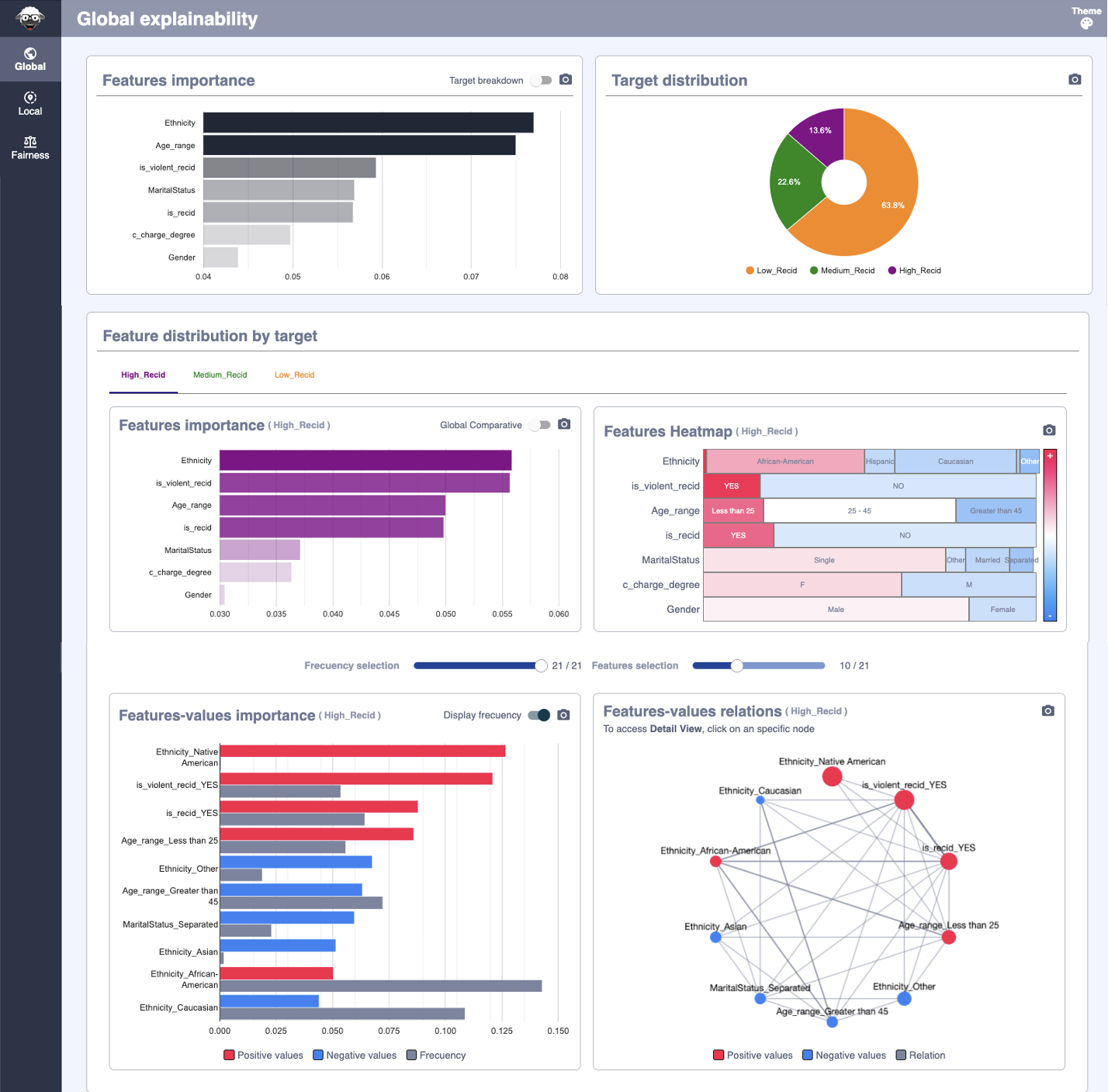
Global Explainability#
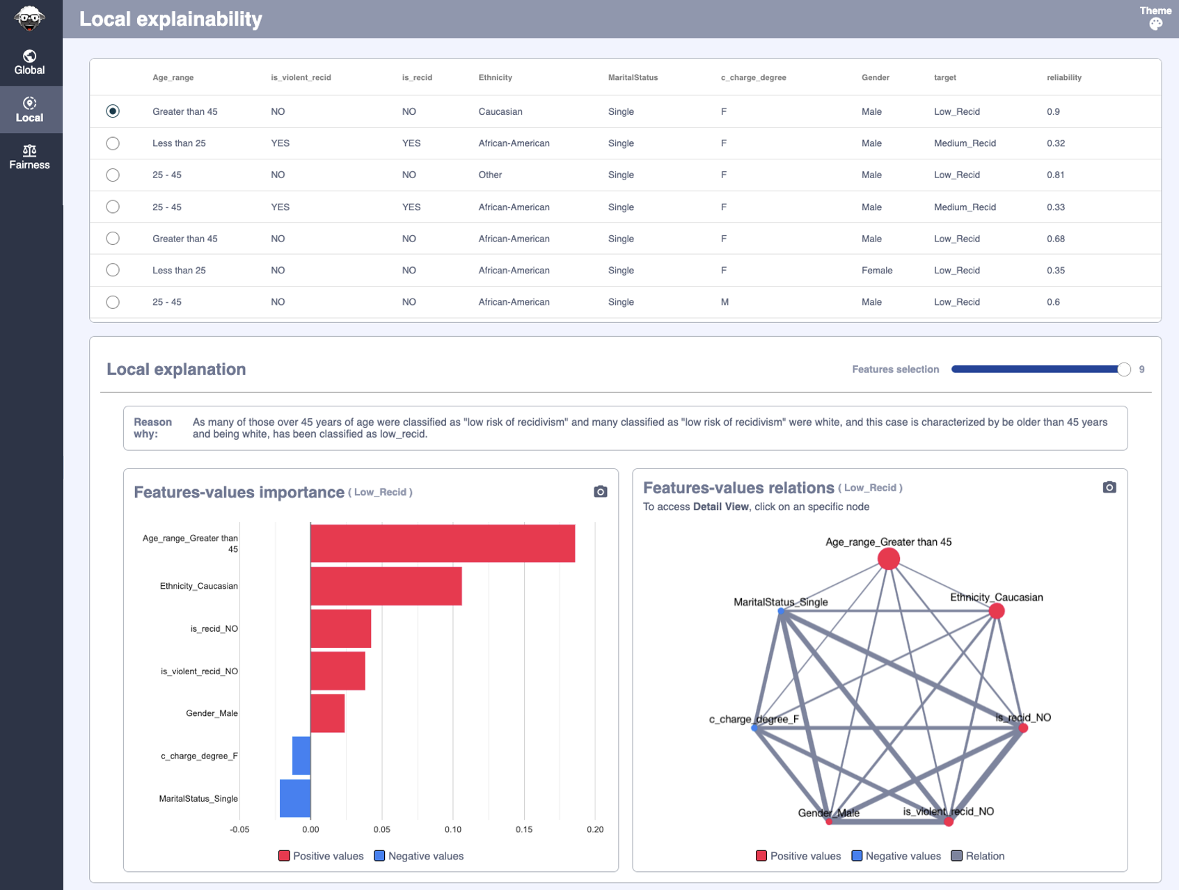
Local Explainability#
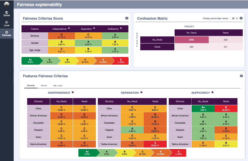
Fairness#