< ✏️ Examples

Body Performance Example

In this example, we use the Body Performace Dataset, that demonstrates how performance levels change with age and some exercise-related features.

This dataset can be obtained using the load_body_performance() function:

>>> from xaiographs.datasets import load_body_performance
>>> df_dataset = load_body_performance()
>>> df_dataset.head(3)
   id   age gender  height_cm  weight_kg  body_fat_%  diastolic  systolic  gripForce  sit_and_bend_forward_cm  sit-ups_counts  broad_jump_cm             class
0   0  27.0      M      172.3      75.24        21.3       80.0     130.0       54.9                     18.4            60.0          217.0   mid_performance
1   1  25.0      M      165.0      55.80        15.7       77.0     126.0       36.4                     16.3            53.0          229.0  high_performance
2   2  31.0      M      179.6      78.00        20.1       92.0     152.0       44.8                     12.0            49.0          181.0   mid_performance

To determine the explainability of this dataset, XAIoGraphs provides a dataset that has already been discretized and columns with targets probabilities using load_body_performance_discretized() function:

>>> from xaiographs.datasets import load_body_performance_discretized
>>> df_dataset, features_cols, target_cols, y_true, y_predict = load_body_performance_discretized()
>>> df_dataset.head(3)
   id    age gender    height_cm  weight_kg body_fat_%  diastolic     systolic  gripForce sit_and_bend_forward_cm sit-ups_counts  broad_jump_cm            y_true         y_predict  high_performance  mid_performance  low_performance
0   0  26-35      M  160-mid-176  55-mid-79  15-mid-30  68-mid-89  115-mid-144    over_47                6-mid-23        over_54    150-mid-229   mid_performance   mid_performance                 0                1                0
1   1    <25      M  160-mid-176  55-mid-79   under_15  68-mid-89  115-mid-144  26-mid-47                6-mid-23      25-mid-54    150-mid-229  high_performance  high_performance                 1                0                0
2   2  26-35      M     over_176  55-mid-79  15-mid-30    over_89     over_144  26-mid-47                6-mid-23      25-mid-54    150-mid-229   mid_performance   mid_performance                 0                1                0

 

Code Example

The following entry point (with Python virtual environment enabled) is used to demonstrate this example.

>> body_performance_example

Alternatively, you may run the code below to view a full implementation of all XAIoGraphs functionalities with this Dataset:

from xaiographs import Explainer
from xaiographs import Fairness
from xaiographs import Why
from xaiographs.datasets import load_body_performance_discretized, load_body_performance_why

LANG = 'en'

# LOAD DATASETS & SEMANTICS
example_dataset, feature_cols, target_cols, y_true, y_predict = load_body_performance_discretized()
df_values_semantics, df_target_values_semantics = load_body_performance_why(language=LANG)

# EXPLAINER
explainer = Explainer(importance_engine='LIDE', number_of_features=11, verbose=1)
explainer.fit(df=example_dataset, feature_cols=feature_cols, target_cols=target_cols)

# WHY
why = Why(language=LANG,
          explainer=explainer,
          why_values_semantics=df_values_semantics,
          why_target_values_semantics=df_target_values_semantics,
          verbose=1)
why.fit()

# FAIRNESS
f = Fairness(verbose=1)
f.fit(df=example_dataset[feature_cols + [y_true] + [y_predict]],
      sensitive_cols=['gender', 'age'],
      target_col=y_true,
      predict_col=y_predict)

 

XAIoWeb Body Performance

After running the .fit() methods of each of the classes (one, two, or all three), a sequence of JSON files are generated in the xaioweb_files folder to visualized in XAIoWeb interface.

To launch the web (with the virtual environment enabled), run the following entry point:

>> xaioweb -d xaioweb_files -o -f

And the results seen in XAIoWeb are the following:

 

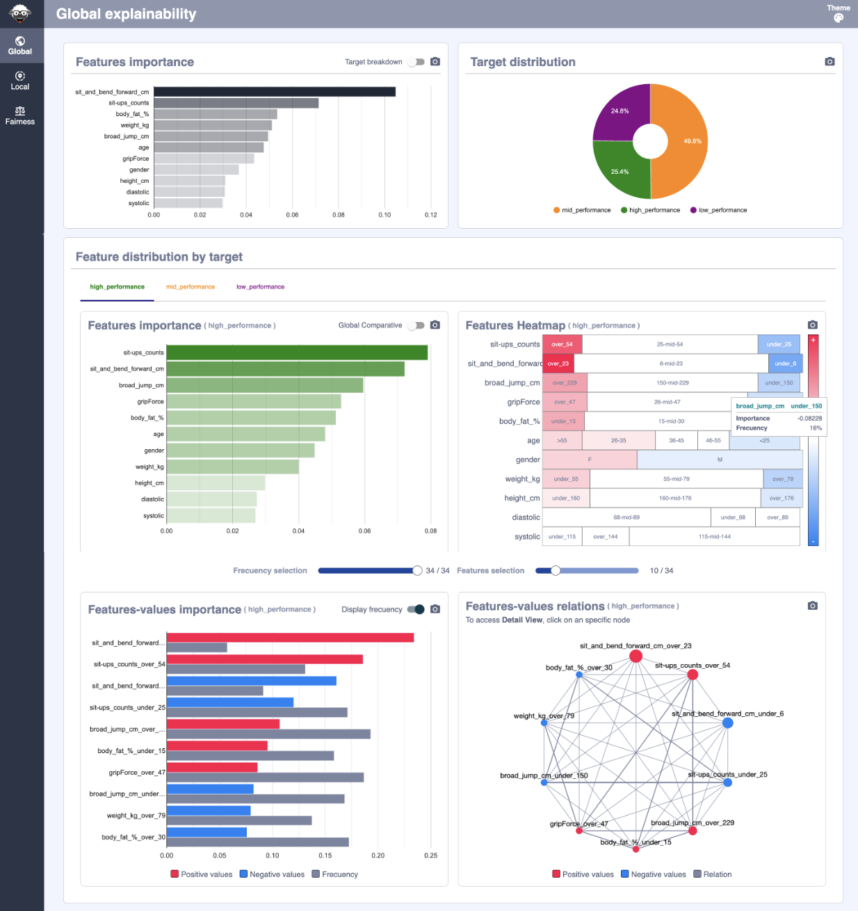
Global Explainability

 

 

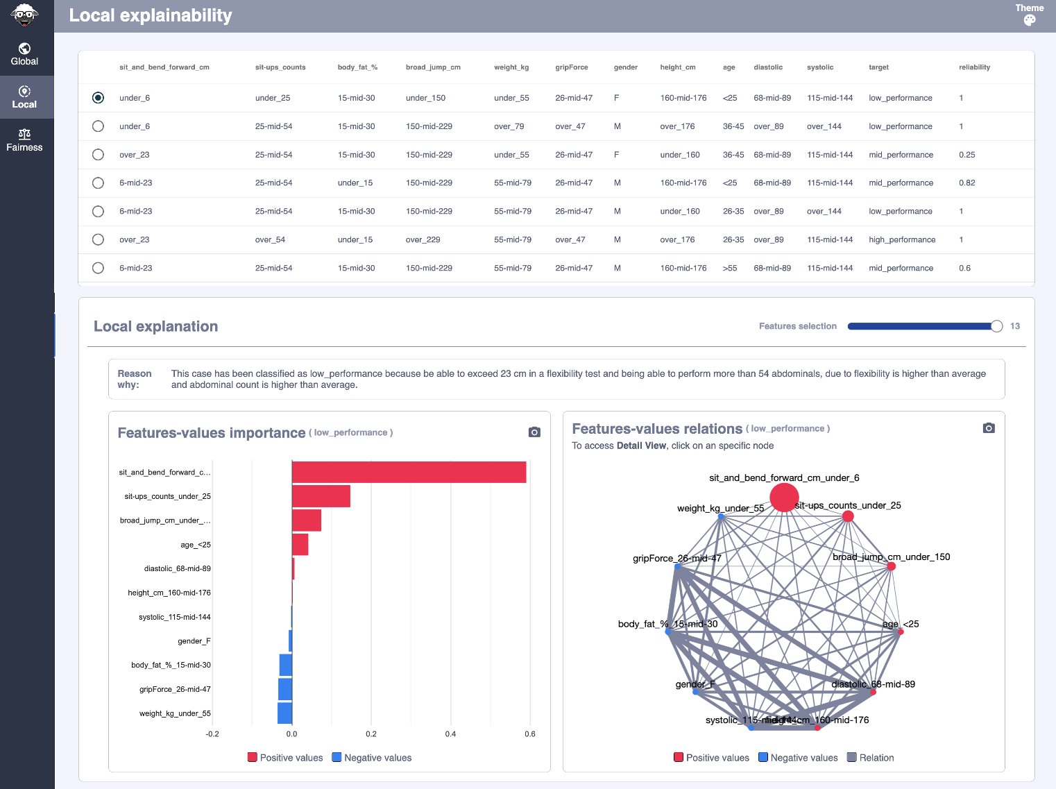
Local Explainability

 

 

Fairness

 

 

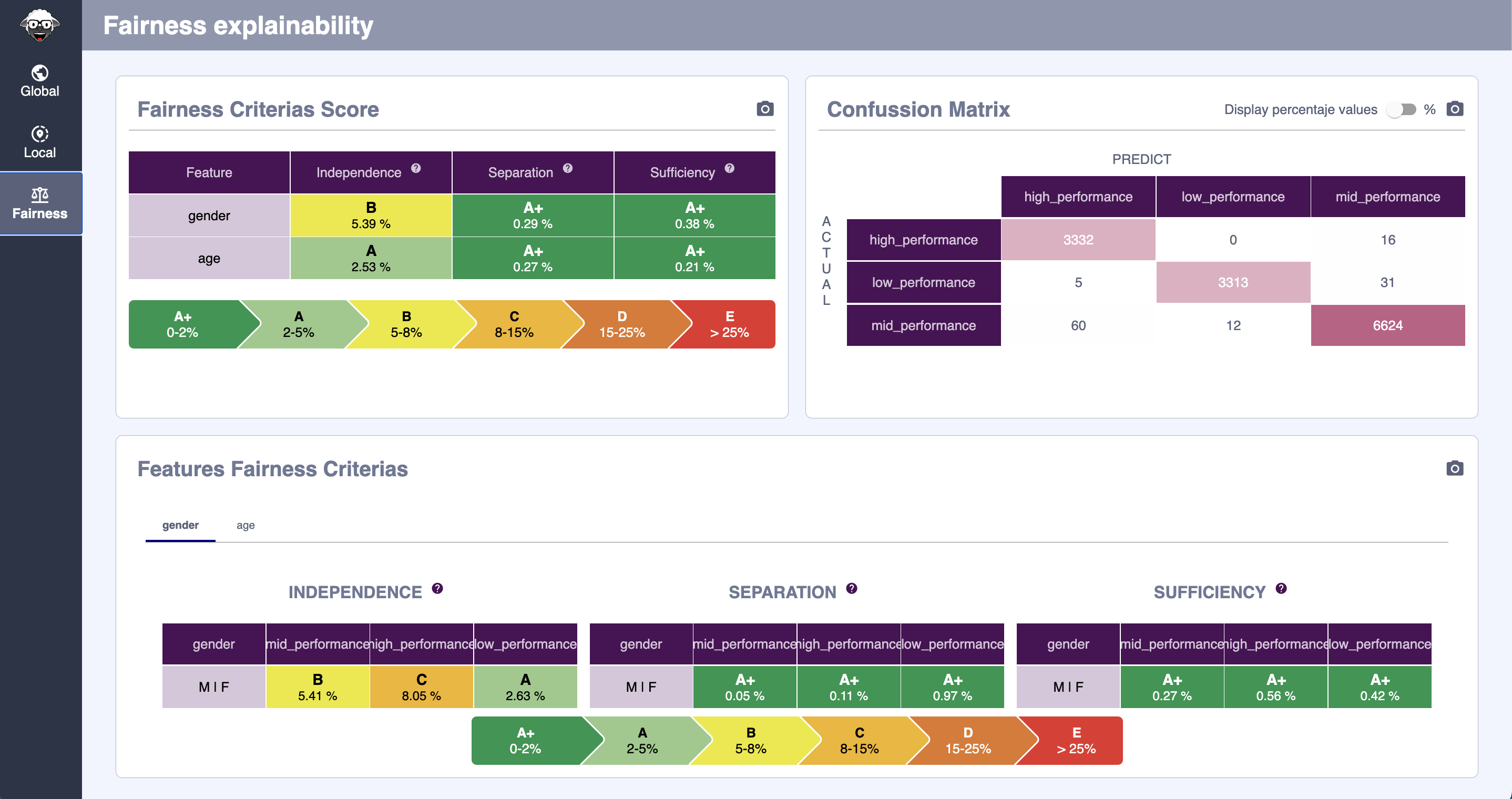
< ✏️ Examples